
1D Motion (Linear Motion)
Now now we have the basics covered, let's get to the good stuff. We're going to start our physics journey with kinematics which is the study of motion. Before we learn about what causes objects to move, we're going to learn how objects move and how to describe the way objects travel through space and time.
We'll begin kinematics by learning about the simplest type of motion: when objects move in a straight line, known as linear motion or one dimensional (1D) motion. Think of a car driving on a straight road or a ball falling down.
Even though linear motion might seem simple, it's really important that we understand the fundamentals because the rest of kinematics (and other sections) builds on what we learn in this lesson. 2D and projectile motion is just linear motion happening in two directions at once. Circular motion is just linear motion wrapped around the circumference of a circle. And rotational motion is just like linear motion but it uses angle units instead of length units.
First we'll cover the basic and essential parts of motion that we'll use for the rest of the course: position, displacement, velocity and acceleration. We'll learn the concepts and the kinematic equations that we can use to analyze and predict the motion of objects, and how to apply every equation to both horizontal and vertical motion. We'll also learn how to create motion graphs.
This lesson will also touch on the difference between scalars and vectors as they relate to kinematics. We're also going to address a common issue many students have when solving physics problems that involve average speed.
1
:
3
0
Position and displacement
9
:
2
3
Velocity
2
2
:
1
1
Acceleration
3
3
:
4
8
Summary
0
:
3
0
Kinematic equations
1
2
:
0
2
Scalars vs vectors
1
9
:
0
7
Average speed problems
2
5
:
4
0
Summary
Now that we have a good understanding of what position, velocity and acceleration are, let's see how these 3 graphs look for different types of motion.
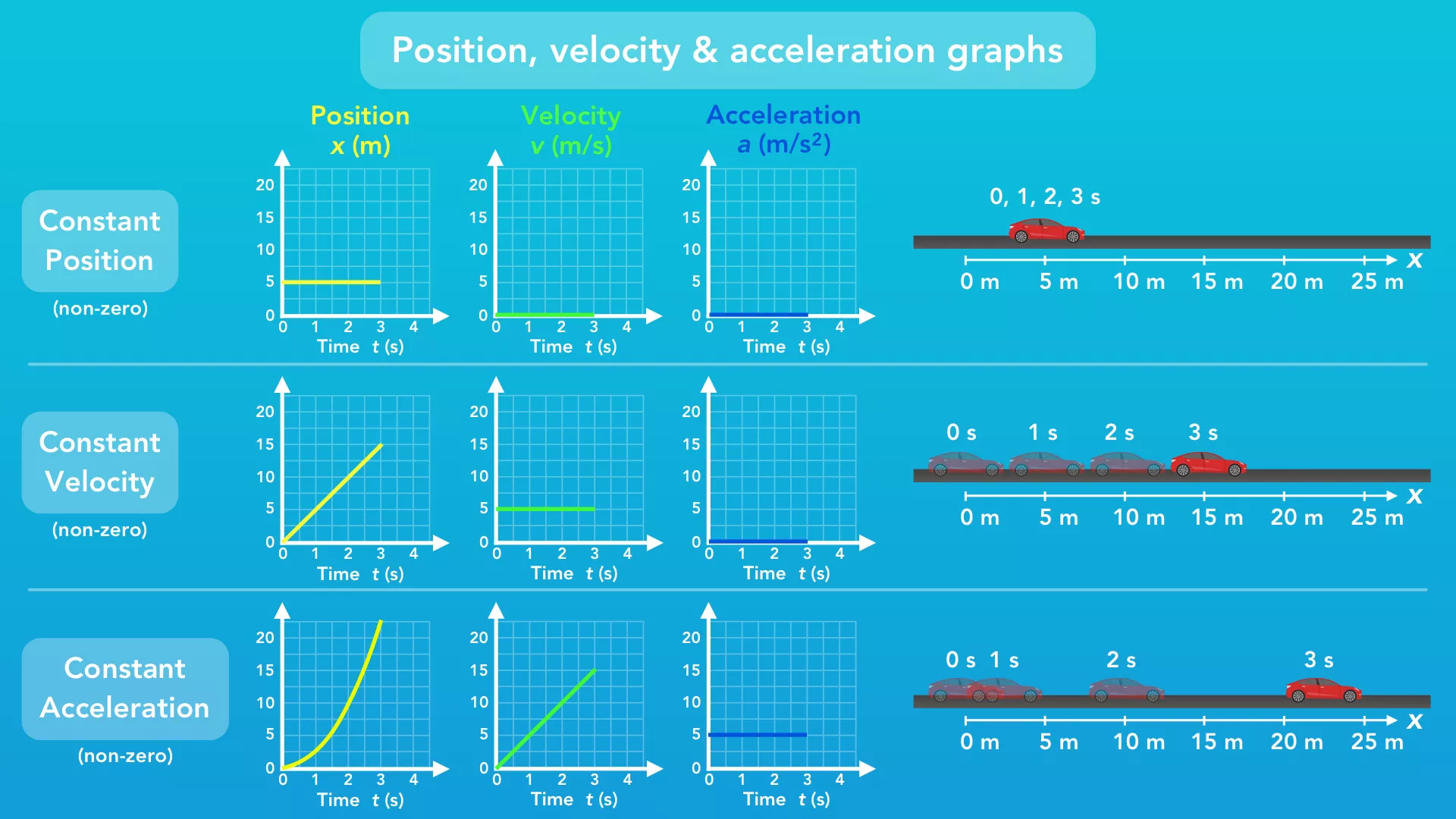
The first row shows the 3 graphs for a car that has a constant position - that means the position doesn't change over time. So really, there's no motion. We can see that the position of the car, and the position graph, remain at 5 m over time (we picked a position other than 0 m to make it more interesting). Since the car is not moving, there is no velocity, so the velocity graph remains at 0 m/s over time. And since that velocity is not changing, the acceleration graph also remains at 0 m/s² over time.
The second row shows the 3 graphs for a car that has a constant velocity. We note that the car has some non-zero velocity because, like for the first car, a constant velocity of 0 m/s is still a constant velocity, and the first row already covers that. So for this 2nd car, we can see from the velocity graph that the car is moving with a constant velocity of 5 m/s over time. Because the velocity is not changing (the car is not speeding up or slowing down), the car has no acceleration. So, the acceleration graph shows 0 m/s² over time. If we look at the position graph, we can see this motion creates a straight line with a positive slope. As the car moves, the position changes over time at a constant rate (slope).
The third row shows the 3 graphs for a car that has a constant acceleration. Like before, note that this car has a non-zero constant acceleration - the previous two cars had a constant acceleration of zero. So starting with the acceleration graph, we see the car has a constant acceleration of 5 m/s² that doesn't change over time. The velocity graph now shows that the velocity is increasing over time. That makes sense - acceleration is change in velocity over time, so the velocity changes over time. Because we have a constant value for acceleration, the velocity increases steadily over time in a straight line. But now when we look at the position graph, we see a curved line. It turns out that if an object is accelerating, the position graph is curved.
So why do we see a curve? How are these 3 graphs related to each other?
The velocity of the object at any point in time is the slope of the position graph, and the acceleration of the object at any point in time is the slope of the velocity graph.
Going the other way, the change in velocity is the area under the acceleration graph, and the change in position is the area under the velocity graph. Let's take a closer look.
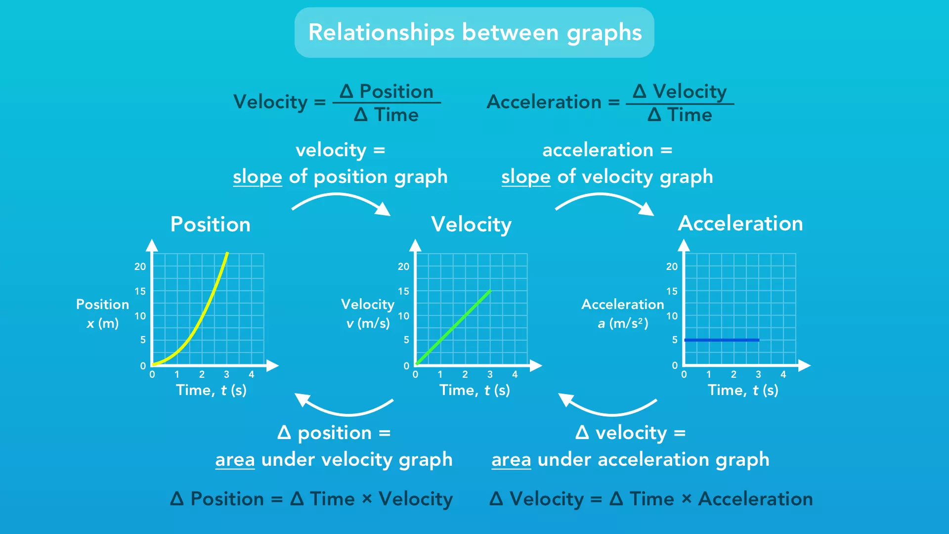
We know that velocity = change in position / change in time. We also know how to find the slope of any line on a graph: slope = change in vertical / change in horizontal. Look similar? Since position is on the vertical axis and time is on the horizontal axis, the slope of the position graph actually gives us the velocity of the object. The same thing goes for velocity and acceleration: since acceleration is the change in velocity over time, the acceleration is the slope of the velocity graph.
If we rearrange our equations, we find: change in position = change in time * velocity. Multiplying time and velocity is actually the same thing as finding the area between the velocity graph line and the horizontal axis. In the specific case of this graph, we see that this area forms a triangle. It's important to realize that this area is equal to the change in position from the initial point to some other point in time. The velocity graph does not tell us what the initial position of the object was, only the change in position. And again, this same thing applies to the velocity and acceleration graphs.
So why is the position graph a curve when we have an acceleration? Well we know that the velocity of the object at an instant in time is the slope of the position graph at that instant in time. And if we have acceleration, the velocity is changing over time, so the slope of the position graph is changing over time. A changing slope will give us a curve, whereas a constant slope gives us a straight line.
Below are two more examples of motion and what the 3 graphs would look like for that motion.


0
:
1
8
Problem 1: Displacement, velocity
8
:
4
4
Problem 2: Displacement, velocity
1
3
:
1
9
Problem 3: Velocity, acceleration
1
7
:
4
9
Problem 4: Position, velocity, acceleration
2
4
:
3
4
Problem 5: Position graph
2
8
:
5
8
Problem 6: Velocity graph
3
2
:
5
4
Problem 7: Velocity graph


Answers

Now now we have the basics covered, let's get to the good stuff. We're going to start our physics journey with kinematics which is the study of motion. Before we learn about what causes objects to move, we're going to learn how objects move and how to describe the way objects travel through space and time.
We'll begin kinematics by learning about the simplest type of motion: when objects move in a straight line, known as linear motion or one dimensional (1D) motion. Think of a car driving on a straight road or a ball falling down.
Even though linear motion might seem simple, it's really important that we understand the fundamentals because the rest of kinematics (and other sections) builds on what we learn in this lesson. 2D and projectile motion is just linear motion happening in two directions at once. Circular motion is just linear motion wrapped around the circumference of a circle. And rotational motion is just like linear motion but it uses angle units instead of length units.
First we'll cover the basic and essential parts of motion that we'll use for the rest of the course: position, displacement, velocity and acceleration. We'll learn the concepts and the kinematic equations that we can use to analyze and predict the motion of objects, and how to apply every equation to both horizontal and vertical motion. We'll also learn how to create motion graphs.
This lesson will also touch on the difference between scalars and vectors as they relate to kinematics. We're also going to address a common issue many students have when solving physics problems that involve average speed.

0 comments